Part 1 was a 9 PM call built on a 6+2 cohort. Part 2 opened up that design: fixed cohort size, active paired with placebo, a stopping rule pre-specified before anyone had real data to argue about.

6+2 is a good design for a specific question: is this dose acceptably safe, given what we’ve seen so far. It is not built to answer a different, harder question that shows up constantly in oncology: which of several doses is both safe enough and effective enough. That second question needs different tools. This post is a survey of two of them — Bayesian Logistic Regression Models (BLRM) and the dose-optimization thinking behind the FDA’s Project Optimus — with a basic implementation so the ideas aren’t just abstract.

This isn’t my daily-driver design the way 6+2 is, so treat this as an introduction and a set of pointers, not a field guide.

Why oncology asks a different question

A 6+2 design works well partly because, in a lot of non-oncology, non-vaccine settings, safety and efficacy can be reasoned about somewhat separately in early phase — get the safety profile right, and a later trial can search for the effective dose with more room to spare.

Oncology often doesn’t have that luxury. Many oncology drugs, especially targeted and immune therapies, don’t follow a simple “more drug, more benefit” curve the way classic chemotherapy roughly does. Pushing to the maximum tolerated dose (MTD) can mean pushing past the dose that actually maximizes benefit, trading tolerability and long-term adherence for a higher number on a dose-escalation chart. That’s the core critique behind the FDA’s Project Optimus, an initiative focused on optimizing dosage to maximize therapeutic benefit while minimizing toxicity.

Two consequences follow:

• Dose-finding needs a model that treats toxicity as a curve across doses, not a pass/fail threshold per cohort — which is what BLRM is built for.
• Dose-finding needs to ask about efficacy and tolerability together, not safety alone — which is what Project Optimus pushes sponsors toward.

BLRM: modeling the dose-toxicity curve directly

A 6+2 cohort review asks, in effect, “did this dose’s data cross a pre-specified line.” A BLRM asks a continuous version of the same question: “given everything we’ve seen across all doses so far, what’s the probability that this dose causes a dose-limiting toxicity (DLT), and how does that change as dose increases.”

The classic form models the probability of DLT at dose \(d\) using a two-parameter logistic curve:

$$ \text{logit}\big(p(d)\big) = \log\alpha + \beta \log(d / d^*) $$

where \(d^*\) is a reference dose, and \(\alpha, \beta\) have priors informed by preclinical data and clinical judgment. As each cohort’s data comes in, the posterior over the whole curve updates — not just the verdict on one dose, but the model’s belief about every dose simultaneously, including ones nobody has tried yet.

A basic BLRM in R and Stan

Dummy data first: a handful of doses, a small number of patients per dose, and a DLT count, simulated under a true (but to the model, unknown) dose-toxicity curve.

library(dplyr)

set.seed(30)

doses <- c(50, 100, 200, 400, 800)
ref_dose <- 200
true_alpha <- 0.3
true_beta <- 1.1

true_p_dlt <- function(d) {
  plogis(log(true_alpha) + true_beta * log(d / ref_dose))
}

n_per_dose <- c(3, 3, 6, 6, 3)

dlt_data <- tibble(
  dose = doses,
  n = n_per_dose,
  true_p = true_p_dlt(doses)
) %>%
  rowwise() %>%
  mutate(dlt = rbinom(1, n, true_p)) %>%
  ungroup()

dlt_data

## # A tibble: 5 × 4
##    dose     n true_p   dlt
##   <dbl> <dbl>  <dbl> <int>
## 1    50     3 0.0613     0
## 2   100     3 0.123      0
## 3   200     6 0.231      1
## 4   400     6 0.391      2
## 5   800     3 0.580      2

Now the Stan model itself. This mirrors the standard two-parameter BLRM, with weakly informative priors on \(\log\alpha\) and \(\log\beta\). Writing the slope as \(\beta = \exp(\log\beta)\) keeps it positive, which forces the toxicity curve to rise monotonically with dose.

blrm_code <- "
data {
  int<lower=1> N;
  vector[N] dose;
  array[N] int<lower=0> n;
  array[N] int<lower=0> dlt;
  real ref_dose;
}
parameters {
  real log_alpha;
  real log_beta;
}
model {
  log_alpha ~ normal(log(0.5), 1);
  log_beta  ~ normal(0, 1);

  for (i in 1:N) {
    real logit_p = log_alpha + exp(log_beta) * log(dose[i] / ref_dose);
    dlt[i] ~ binomial_logit(n[i], logit_p);
  }
}
generated quantities {
  vector[N] p_dlt;
  for (i in 1:N) {
    p_dlt[i] = inv_logit(log_alpha + exp(log_beta) * log(dose[i] / ref_dose));
  }
}
"

library(rstan)
rstan_options(auto_write = TRUE)

stan_data <- list(
  N = nrow(dlt_data),
  dose = dlt_data$dose,
  n = dlt_data$n,
  dlt = dlt_data$dlt,
  ref_dose = ref_dose
)

blrm_fit <- stan(
  model_code = blrm_code,
  data = stan_data,
  iter = 2000,
  warmup = 1000,
  chains = 4,
  cores = 4,
  seed = 42
)

print(blrm_fit, pars = c("log_alpha", "log_beta"))

## Inference for Stan model: anon_model.
## 4 chains, each with iter=2000; warmup=1000; thin=1; 
## post-warmup draws per chain=1000, total post-warmup draws=4000.
## 
##            mean se_mean   sd  2.5%  25%   50%   75% 97.5% n_eff Rhat
## log_alpha -1.44    0.01 0.54 -2.55 -1.8 -1.42 -1.07 -0.42  1445    1
## log_beta   0.12    0.02 0.62 -1.40 -0.2  0.22  0.55  1.05  1254    1
## 
## Samples were drawn using NUTS(diag_e) at Sat Jun 27 17:53:19 2026.
## For each parameter, n_eff is a crude measure of effective sample size,
## and Rhat is the potential scale reduction factor on split chains (at 
## convergence, Rhat=1).

library(ggplot2)

p_dlt_summary <- summary(blrm_fit, pars = "p_dlt")$summary %>%
  as_tibble() %>%
  mutate(dose = doses)

ggplot(p_dlt_summary, aes(x = dose, y = mean)) +
  geom_ribbon(aes(ymin = `2.5%`, ymax = `97.5%`), alpha = 0.2) +
  geom_line(linewidth = 1) +
  geom_point(data = dlt_data, aes(x = dose, y = dlt / n), color = "firebrick", size = 2) +
  scale_x_log10() +
  labs(
    title = "Posterior dose-toxicity curve (BLRM)",
    subtitle = "Shaded band: 95% credible interval. Red points: observed DLT rate by dose.",
    x = "Dose (log scale)",
    y = "P(DLT)"
  ) +
  theme_minimal()

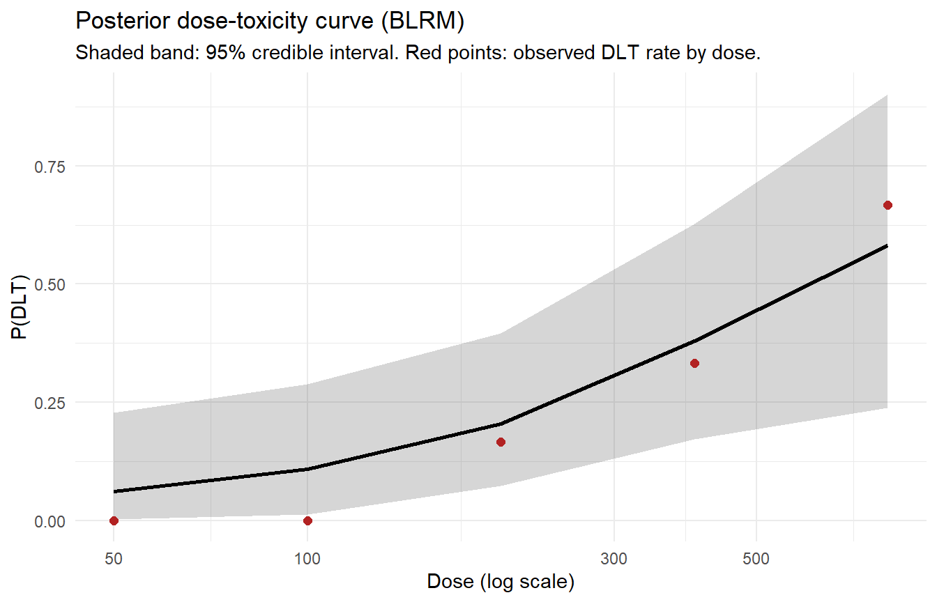
Running this needs rstan and a one-time model compilation, but the payoff is the whole point: the output is a full posterior curve across all five doses, not five independent yes/no verdicts. That’s the structural difference from 6+2 — a 6+2 cohort review never tells you anything about a dose nobody has tried yet, whereas a BLRM, by sharing information across doses through the shared \(\alpha, \beta\) parameters, does. Notice too how the credible band fans out at the top dose, where only a handful of patients have been treated: the model stays honest about how little it knows out there instead of reporting a single confident number.

This is also the point where, operationally, a BLRM-based trial typically layers an Escalation with Overdose Control (EWOC) rule on top — choosing the next dose as the highest one whose posterior probability of excessive toxicity stays under a pre-specified ceiling. I’m leaving that out of the code here to keep the post focused, but it’s the natural next step if you build on this.

Project Optimus: asking the other half of the question

A BLRM, on its own, still only answers a safety question — a more flexible one than 6+2, but a safety question. Project Optimus represents a shift in the FDA’s approach to dose selection in oncology, moving away from the maximum tolerated dose toward an optimal biological dose — the dose that delivers benefit with acceptable toxicity, not just the highest dose patients can tolerate.

Practically, the resulting guidance generally points sponsors toward carrying two doses — the MTD and a dose below it — into a later randomized comparison to see which one actually performs better once both safety and efficacy are considered together, rather than assuming the higher dose automatically wins.

That has a few downstream effects worth knowing even outside oncology:

• Dose-finding stops being a single escalating ladder and starts looking like a small randomized comparison between candidate doses.
• Sponsors are expected to support dose decisions with mechanistic and clinical evidence, not toxicity data alone.
• Trial timelines and sample sizes grow, since you’re no longer stopping the moment you find a tolerable ceiling.

None of this replaces 6+2-style designs where the dose-response question is simpler and the safety question really is closer to the only question. It’s a reminder that the right early-phase design depends on what kind of curve you actually expect the drug to have — flat-ish efficacy past some dose plus rising toxicity calls for something like BLRM-with-randomized-comparison; a more conventional dose-response relationship can be served well by something as direct as 6+2.

Closing the series

Across these three posts: a 9 PM call built on incomplete information, the 6+2 structure that made that call possible to have at all, and now a look at what changes when the question gets harder. The common thread is the one from Part 1 — the statistical work that matters most in early-phase trials isn’t the test run after the data arrives, it’s the design decided weeks before, built to hold up under exactly the kind of pressure a real cohort eventually brings.

That’s where I’ll leave the series for now. If you’d want me to go deeper on any of it — EWOC in practice, fitting a BLRM end to end, or how Project Optimus is playing out in real submissions — let me know and I’ll pick it back up.

💬 Found this series useful? I’d be glad to hear your take on LinkedIn and tag me.

This post uses entirely simulated data and references publicly available regulatory guidance. No real trial, patient, or molecule is represented.