In critical applications like healthcare, knowing the probability isn’t enough. Knowing how confident we are in that probability makes all the difference.

🔍 The Problem

Diabetes prediction models abound, but they often give us just a number. Traditional classifiers like logistic regression or random forests will tell you, for instance, that there’s a 73% chance someone has diabetes.

But what if we asked:

“How sure are we about that 73%?”

Enter Bayesian Neural Networks (bnns), where uncertainty isn’t a bug—it’s a feature.

📊 The Data

We used the PimaIndiansDiabetes2 dataset from the mlbench package, containing clinical variables (e.g., glucose, BMI, insulin) and diabetes diagnosis. Missing values were removed, and outcomes were converted to binary.

library(bnns)
library(mlbench)
library(rsample)
library(ggplot2)

set.seed(123)
data("PimaIndiansDiabetes2")
trial_data <- PimaIndiansDiabetes2 |>
  transform(diabetes = ifelse(diabetes == "pos", 1, 0)) |>
  na.omit()

trial_data_split <- initial_split(trial_data, strata = diabetes, prop = 0.8)
trial_data_train <- training(trial_data_split)
trial_data_test <- testing(trial_data_split)

🧠 The Model

Our BNN has two hidden layers (24 and 12 nodes) and uses Cauchy priors to encourage sparsity. We used logistic output activation (out_act_fn = 2) for binary classification.

bnn_model <- bnns(
  diabetes ~ .,
  data = trial_data_train,
  L = 2,
  nodes = c(24, 12),
  act_fn = c(4, 1),
  out_act_fn = 2,
  iter = 0.1e4,
  warmup = 0.05e4,
  chains = 4,
  cores = 4,
  prior_weights = list(dist = "cauchy", params = list(mu = 0, sigma = 0.3)),
  prior_bias = list(dist = "cauchy", params = list(mu = 0, sigma = 0.3))
)

🎯 The Prediction

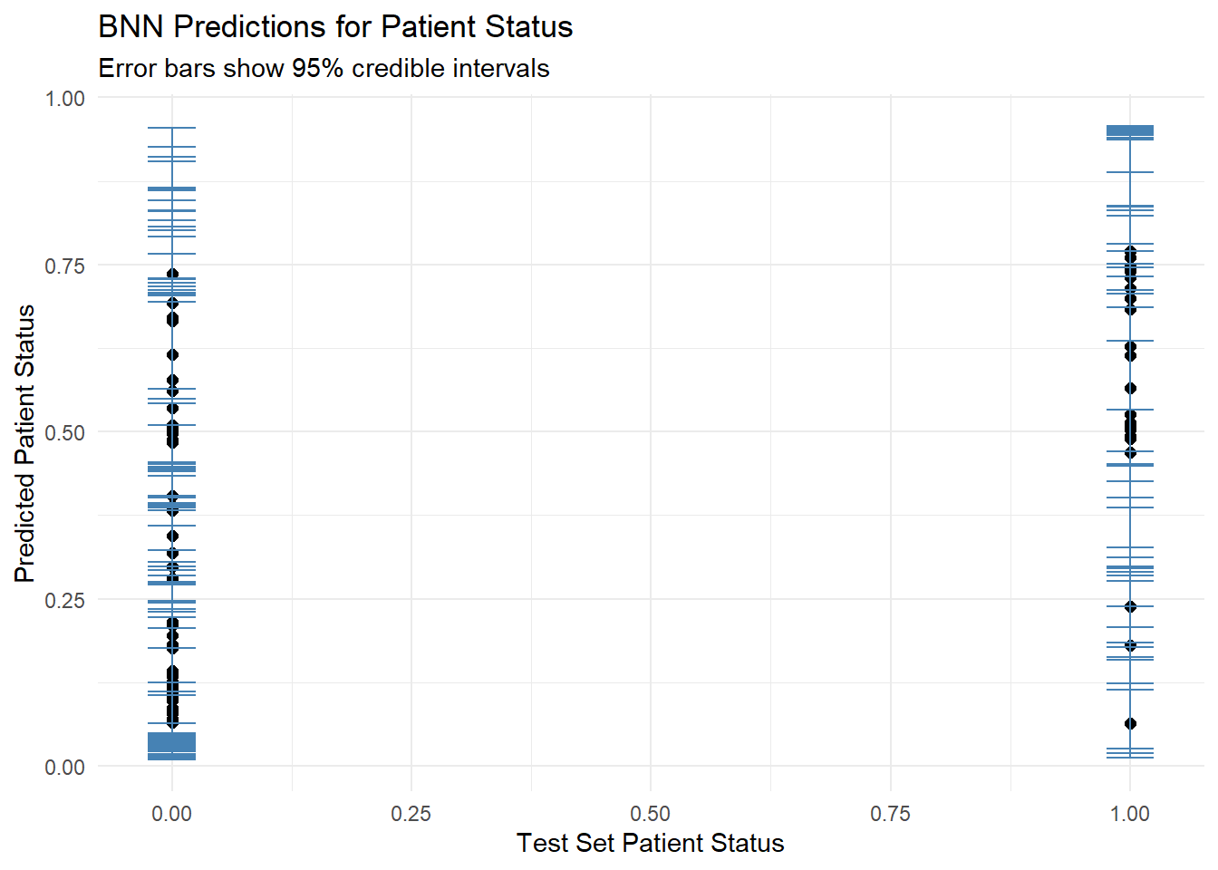
We predicted probabilities on the test set and extracted the posterior median and 95% credible intervals.

pred <- predict(bnn_model, newdata = trial_data_test)
pred_y <- apply(pred, MARGIN = 1, median)
pred_quantiles <- apply(pred, 1, function(x) quantile(x, probs = c(0.025, 0.975)), simplify = FALSE) |>
  do.call(rbind, args = _)

📏 Model Performance

measure_bin(trial_data_test$diabetes, pred)

Setting levels: control = 0, case = 1

Setting direction: controls < cases

$conf_mat
   pred_label
obs  0  1
  0 42 11
  1  7 19

$accuracy
[1] 0.7721519

$ROC

Call:
roc.default(response = obs, predictor = pred)

Data: pred in 53 controls (obs 0) < 26 cases (obs 1).
Area under the curve: 0.8353

$AUC
[1] 0.8352685

Performance was comparable to classical methods (AUC ~0.835), but with a massive advantage: uncertainty quantification.

🔬 Visualizing Predictions

plot_data <- data.frame(
  Actual = trial_data_test$diabetes,
  Predicted = pred_y,
  Lower = pred_quantiles[,1],
  Upper = pred_quantiles[,2]
) |>
  transform(width = Upper - Lower) |>
  dplyr::arrange(width)

ggplot(plot_data, aes(x = Actual, y = Predicted)) +
  geom_point(size = 2) +
  geom_errorbar(aes(ymin = Lower, ymax = Upper), width = 0.05, color = "steelblue") +
  labs(
    title = "BNN Predictions for Patient Status",
    subtitle = "Error bars show 95% credible intervals",
    x = "Test Set Patient Status",
    y = "Predicted Patient Status"
  ) +
  theme_minimal()

🧠 Why Use bnns?

1. Non-linear modeling: Captures complex relationships among covariates without heavy pre-specification.
2. Credible intervals: Each prediction comes with its uncertainty.
3. Probability of a probability:
   • For example: Pr(Pr(Diabetes) > 0.5) > 0.9
   • Translation: “We are 90% confident this person has more than 50% risk.”
   • That’s clinical-grade insight.

📣 Final Thoughts

Bayesian Neural Networks let us move beyond binary thinking and embrace informed uncertainty. When the stakes are high (think medicine, finance, or policy), bnns offers a probabilistic flashlight in the black box jungle.

Ready to stop guessing your predictions? Start modeling your belief about your predictions.

🔗 Explore the bnns package

💬 Like this blog? Share your thoughts and use-cases on LinkedIn and tag me!