Using bnns for TMLE

Introduction

This document demonstrates how to use the bnns package with TMLE for causal inference. TMLE combines machine learning-based flexible models with statistical principles to produce unbiased and efficient estimators of causal effects, such as the Average Treatment Effect (ATE). The example also highlights how the flexibility of Bayesian Neural Networks (BNNs) can improve TMLE results when handling complex data-generating mechanisms. This tutorial borrows from this tmle tutorial.

Simulating Data

We simulate data where the treatment assignment and outcome are influenced by multiple covariates, and the true ATE is known.

library(bnns)

# Set a random seed for reproducibility
set.seed(123)

# Simulate data
n <- 1000  # Number of samples
X1 <- rnorm(n)
X2 <- rnorm(n)
U <- rbinom(n, 1, 0.5)  # Unmeasured confounder

# Treatment mechanism (biased by U)
ps <- plogis(0.5 * X1 - 0.5 * X2 + 0.8 * U)
A <- rbinom(n, 1, ps)  # Treatment assignment

# Outcome mechanism (non-linear and confounded by U)
Y_prob <- plogis(1 + 2 * X1^2 - 1.5 * X2 + 1.2 * A + 1.5 * U)
Y <- rbinom(n, 1, Y_prob)

# Combine into a dataset
sim_data <- data.frame(Y, A, X1, X2)

# True ATE for comparison
true_ate <- mean(plogis(1 + 2 * X1^2 - 1.5 * X2 + 1.2 * 1 + 1.5 * U)) -
  mean(plogis(1 + 2 * X1^2 - 1.5 * X2 + 1.2 * 0 + 1.5 * U))
true_ate
#> [1] 0.07431068

Applying TMLE with `bnns`

Step 1: Install and Load Required Packages

Ensure that the bnns and tmle packages are installed.

# Install ggplot2 and bnns from CRAN
# install.packages("ggplot2")
# install.packages("bnns")

Step 2: TMLE Implementation

We use tmle to estimate the ATE. Both the treatment mechanism (g) and the outcome mechanism (Q) are modeled using Bayesian Neural Networks via the bnns package.

### Step 1: Estimate Q
Q <- bnns(Y ~ -1 + ., data = sim_data, L = 2, nodes = c(2, 2), act_fn = c(2, 2), out_act_fn = 2)

Q_A <- predict(Q) # obtain predictions for everyone using the treatment they actually received
sim_data_1 <- sim_data |> transform(A = 1)  # data set where everyone received treatment
Q_1 <- predict(Q, newdata = sim_data_1) # predict on that everyone-exposed data set
sim_data_0 <- sim_data |> transform(A = 0) # data set where no one received treatment
Q_0 <- predict(Q, newdata = sim_data_0)
dat_tmle <- lapply(1:dim(Q_A)[2], function(i) data.frame(Y = sim_data$Y, A = sim_data$A, Q_A = Q_A[,i], Q_0 = Q_0[,i], Q_1 = Q_1[,i]))

### Step 2: Estimate g and compute H(A,W)
g <- bnns(A ~ -1 + . - Y, data = sim_data, L = 2, nodes = c(2, 2), act_fn = c(2, 2), out_act_fn = 2)

g_w <- predict(g) # Pr(A=1|W)
H_1 <- 1/g_w
H_0 <- -1/(1-g_w) # Pr(A=0|W) is 1-Pr(A=1|W)
dat_tmle <- # add clever covariate data to dat_tmle
  lapply(1:dim(Q_A)[2], function(i) dat_tmle[[i]] |>
           cbind(
             H_1 = H_1[,i],
             H_0 = H_0[,i]) |>
           transform(H_A = ifelse(A == 1, H_1, # if A is 1 (treated), assign H_1
                               H_0))  # if A is 0 (not treated), assign H_0
  )

### Step 3: Estimate fluctuation parameter
tmle_ate_list <- lapply(1:dim(Q_A)[2], function(i){
  glm_fit <- glm(Y ~ -1 + offset(qlogis(Q_A)) + H_A, data=dat_tmle[[i]], family=binomial) # fixed intercept logistic regression
  eps <- coef(glm_fit) # save the only coefficient, called epsilon in TMLE lit
  
  ### Step 4: Update Q's
  Q_A_update <- with(dat_tmle[[i]], plogis(qlogis(Q_A) + eps*H_A)) # updated expected outcome given treatment actually received
  Q_1_update <- with(dat_tmle[[i]], plogis(qlogis(Q_1) + eps*H_1)) # updated expected outcome for everyone receiving treatment
  Q_0_update <- with(dat_tmle[[i]], plogis(qlogis(Q_0) + eps*H_0)) # updated expected outcome for everyone not receiving treatment
  
  ### Step 5: Compute ATE
  tmle_ate <- mean(Q_1_update - Q_0_update) # mean diff in updated expected outcome estimates  
  return(tmle_ate)
})

tmle_ate <- unlist(tmle_ate_list)
median(tmle_ate)
#> [1] 0.08953815

Comparing TMLE to Traditional Methods

To highlight the benefits of TMLE, compare it to other methods such as:

IPTW (Inverse Probability of Treatment Weighting)
Naive Comparison (Unadjusted Difference in Means)

library(tmle)
#> Loading required package: glmnet
#> Loading required package: Matrix
#> Loaded glmnet 4.1-8
#> Loading required package: SuperLearner
#> Loading required package: nnls
#> Loading required package: gam
#> Loading required package: splines
#> Loading required package: foreach
#> Loaded gam 1.22-5
#> Super Learner
#> Version: 2.0-29
#> Package created on 2024-02-06
#> Welcome to the tmle package, version 2.0.1.1
#> 
#> Use tmleNews() to see details on changes and bug fixes
freq_tmle <- tmle(
  Y = sim_data$Y, A = sim_data$A, 
  W = sim_data[, c("X1", "X2")], 
  Q.SL.library = c("SL.glm", "SL.ranger"),
  g.SL.library = c("SL.glm", "SL.ranger")
)
#> Loading required namespace: ranger

# Results
freq_tmle_ate <- freq_tmle$estimates$ATE$psi

# Naive Comparison
naive_ate <- mean(sim_data$Y[sim_data$A == 1]) - mean(sim_data$Y[sim_data$A == 0])

# Summary of Results
results <- data.frame(
  Method = c("True ATE", "BNN_TMLE", "Freq_TMLE", "Naive"),
  Estimate = c(true_ate, median(tmle_ate), freq_tmle_ate, naive_ate),
  CI_low = c(true_ate, quantile(tmle_ate, probs = c(0.025)), freq_tmle$estimates$ATE$CI[1], naive_ate),
  CI_high = c(true_ate, quantile(tmle_ate, probs = c(0.975)), freq_tmle$estimates$ATE$CI[2], naive_ate)
)
results
#>      Method   Estimate     CI_low    CI_high
#> 1  True ATE 0.07431068 0.07431068 0.07431068
#> 2  BNN_TMLE 0.08953815 0.08375025 0.09581528
#> 3 Freq_TMLE 0.09309979 0.05910546 0.12709413
#> 4     Naive 0.12824940 0.12824940 0.12824940

Visualizing Results

Plot the estimates from different methods to compare their performance.

library(ggplot2)

ggplot(results, aes(x = forcats::fct_reorder(Method, Estimate), y = Estimate, fill = Method)) +
  geom_bar(stat = "identity", color = "black") +
  geom_hline(yintercept = true_ate, linetype = "dashed", color = "red") +
  geom_errorbar(mapping = aes(ymin = CI_low, ymax = CI_high)) +
  labs(
    title = "Comparison of ATE Estimates",
    y = "ATE Estimate",
    x = "Method"
  ) +
  theme_minimal() +
  theme(legend.position = "none")

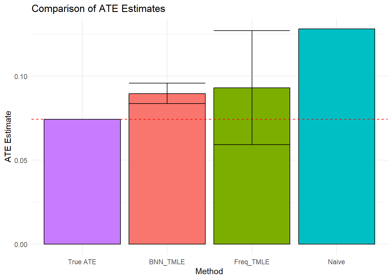
Summary

This tutorial demonstrates how to use the bnns package for TMLE to estimate the Average Treatment Effect (ATE). By leveraging the flexibility of Bayesian Neural Networks, TMLE can handle complex data structures and improve accuracy compared to traditional methods. Use this workflow for applications in clinical trials, epidemiology, and other domains requiring robust causal inference.