Introduction
This presentation explores the performance differences between base R and the dplyr package for various data manipulation tasks.
- While dplyr is renowned for its intuitive syntax and efficiency,
- base R functions can sometimes outperform it, particularly in large simulations.
Understanding these differences can aid in making informed decisions when choosing data wrangling techniques.
The Iris Dataset
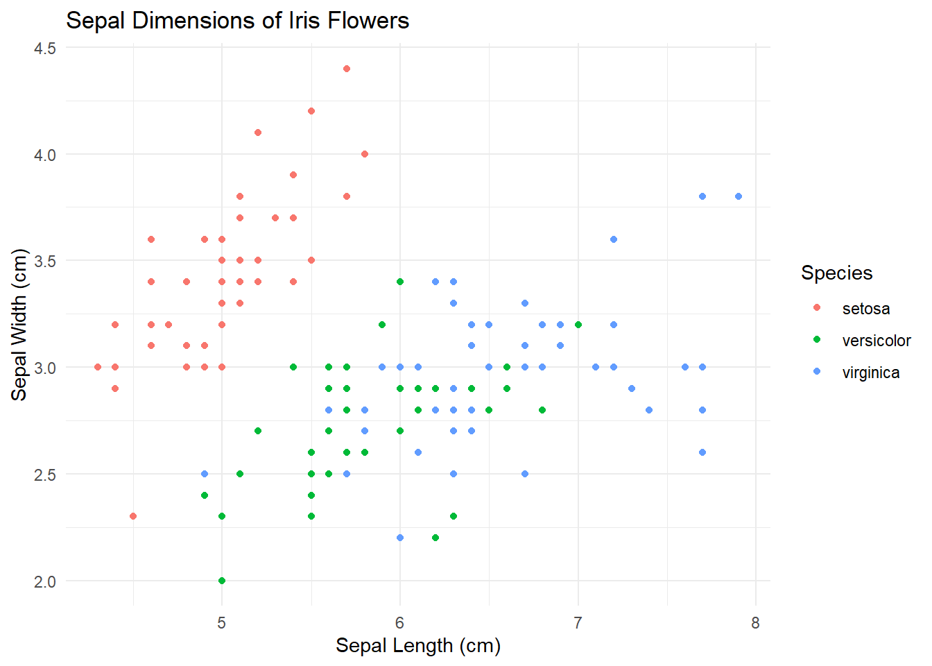
The iris dataset is a classic dataset in statistics and machine learning, often used for demonstrating data manipulation and analysis techniques.
It contains measurements of flower characteristics for three species of iris: setosa, versicolor, and virginica.
Key Features:
150 observations: 50 samples for each species.
4 numeric attributes: Sepal.Length, Sepal.Width, Petal.Length, Petal.Width
1 categorical attribute: Species: The species of the iris flower (setosa, versicolor, virginica).
The Iris Dataset (continued)
    Sepal.Length Sepal.Width Petal.Length Petal.Width    Species
1            5.1         3.5          1.4         0.2     setosa
2            4.9         3.0          1.4         0.2     setosa
3            4.7         3.2          1.3         0.2     setosa
51           7.0         3.2          4.7         1.4 versicolor
52           6.4         3.2          4.5         1.5 versicolor
53           6.9         3.1          4.9         1.5 versicolor
101          6.3         3.3          6.0         2.5  virginica
102          5.8         2.7          5.1         1.9  virginica
103          7.1         3.0          5.9         2.1  virginica
Benchmarking Data Manipulation Tasks
1. Filter Rows
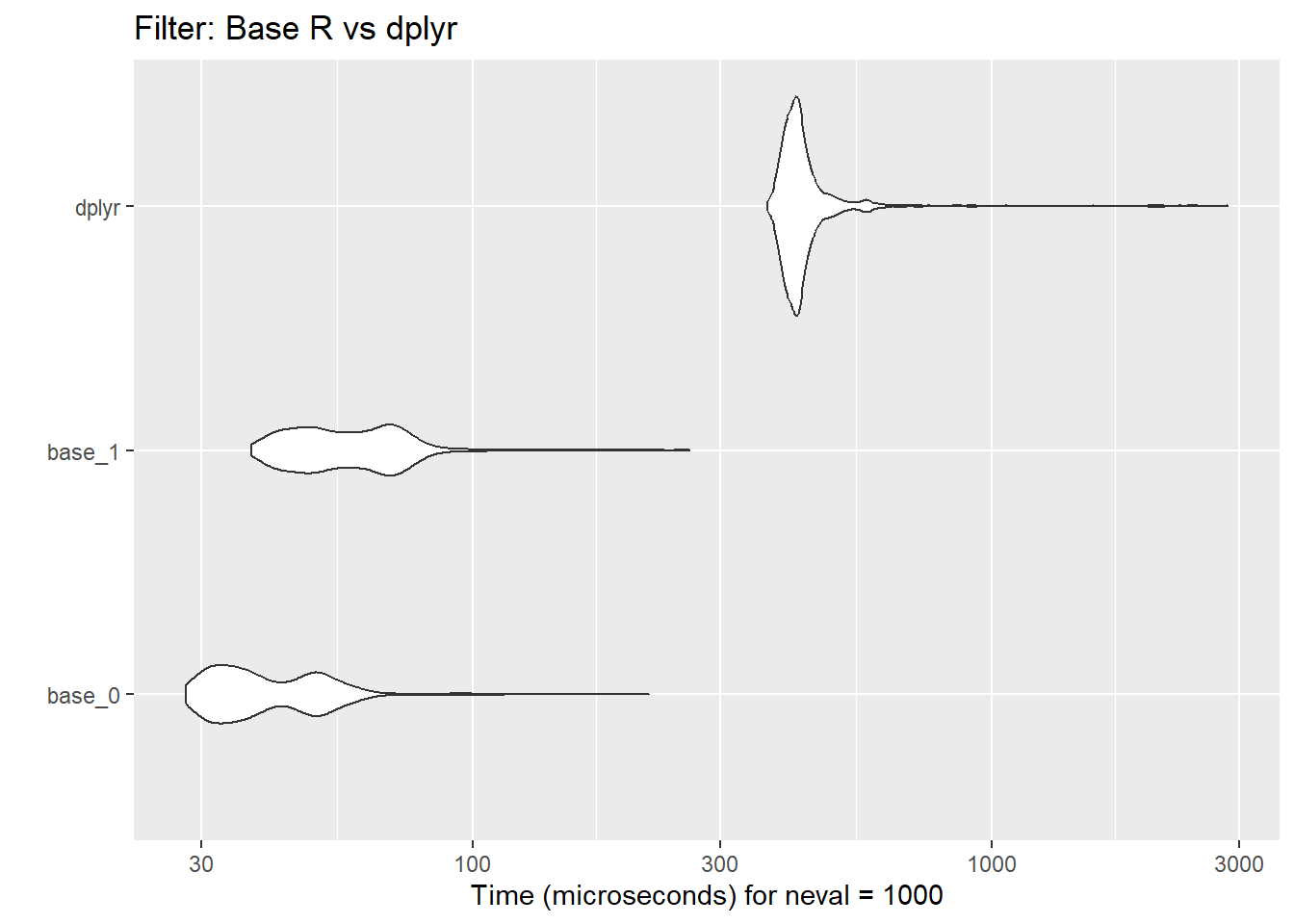
Filtering rows is a common operation in data analysis. This section benchmarks the efficiency of base R’s subsetting approaches against the dplyr::filter function. While dplyr provides clean syntax, base R’s performance is more efficient.
mcb_filter <- microbenchmark(
base_0 = iris[iris$Species == "setosa", ],
base_1 = subset(iris, Species == "setosa"),
dplyr = filter(iris, Species == "setosa"),
times = 1e3
)
mcb_filter
Unit: microseconds
   expr   min     lq     mean median    uq    max neval cld
 base_0  28.0  32.70  42.0561  37.90  49.5  218.6  1000 a
 base_1  37.5  46.95  59.3593  56.65  68.8  261.2  1000  b
  dplyr 369.9 404.85 451.8073 421.30 440.1 2846.6  1000   c
autoplot(mcb_filter) + ggtitle("Filter: Base R vs dplyr")
agg_filter <- aggregate(time ~ expr, data = data.frame(mcb_filter), mean)$time
So, base R code is on average 11 times faster than dplyr::filter. The absolute difference in 10k simulations is 4.097512 seconds.
2. Select Columns
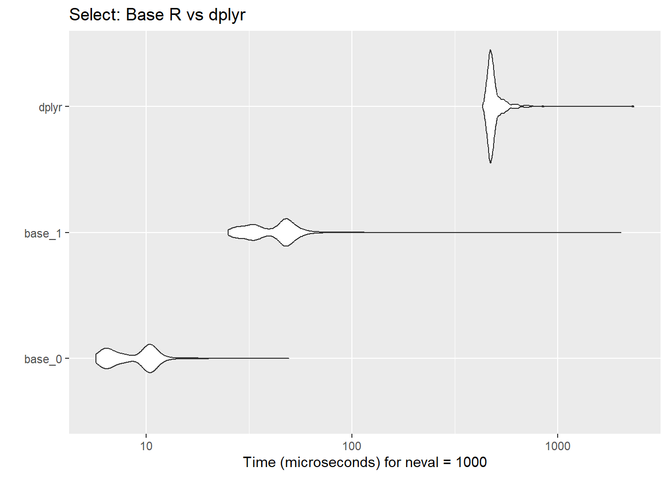
Selecting specific columns is fundamental to narrowing down datasets. The comparison here shows how base R indexing and the subset function stack up against dplyr::select in terms of speed.
mcb_select <- microbenchmark(
base_0 = iris[, c("Sepal.Length", "Petal.Length")],
base_1 = subset(iris, select = c(Sepal.Length, Petal.Length)),
dplyr = select(iris, Sepal.Length, Petal.Length),
times = 1e3
)
mcb_select
Unit: microseconds
   expr   min     lq     mean median    uq    max neval cld
 base_0   5.7   6.65   9.0531   9.60  10.6   49.3  1000 a
 base_1  25.1  32.60  43.7883  44.75  48.6 2026.9  1000  b
  dplyr 433.1 465.30 498.3363 478.00 497.7 2342.9  1000   c
autoplot(mcb_select) + ggtitle("Select: Base R vs dplyr")
agg_select <- aggregate(time ~ expr, data = data.frame(mcb_select), mean)$time
So, base R code is on average 55 times faster than dplyr::select. The absolute difference in 10k simulations is 4.892832 seconds.
3. Add/Modify Columns
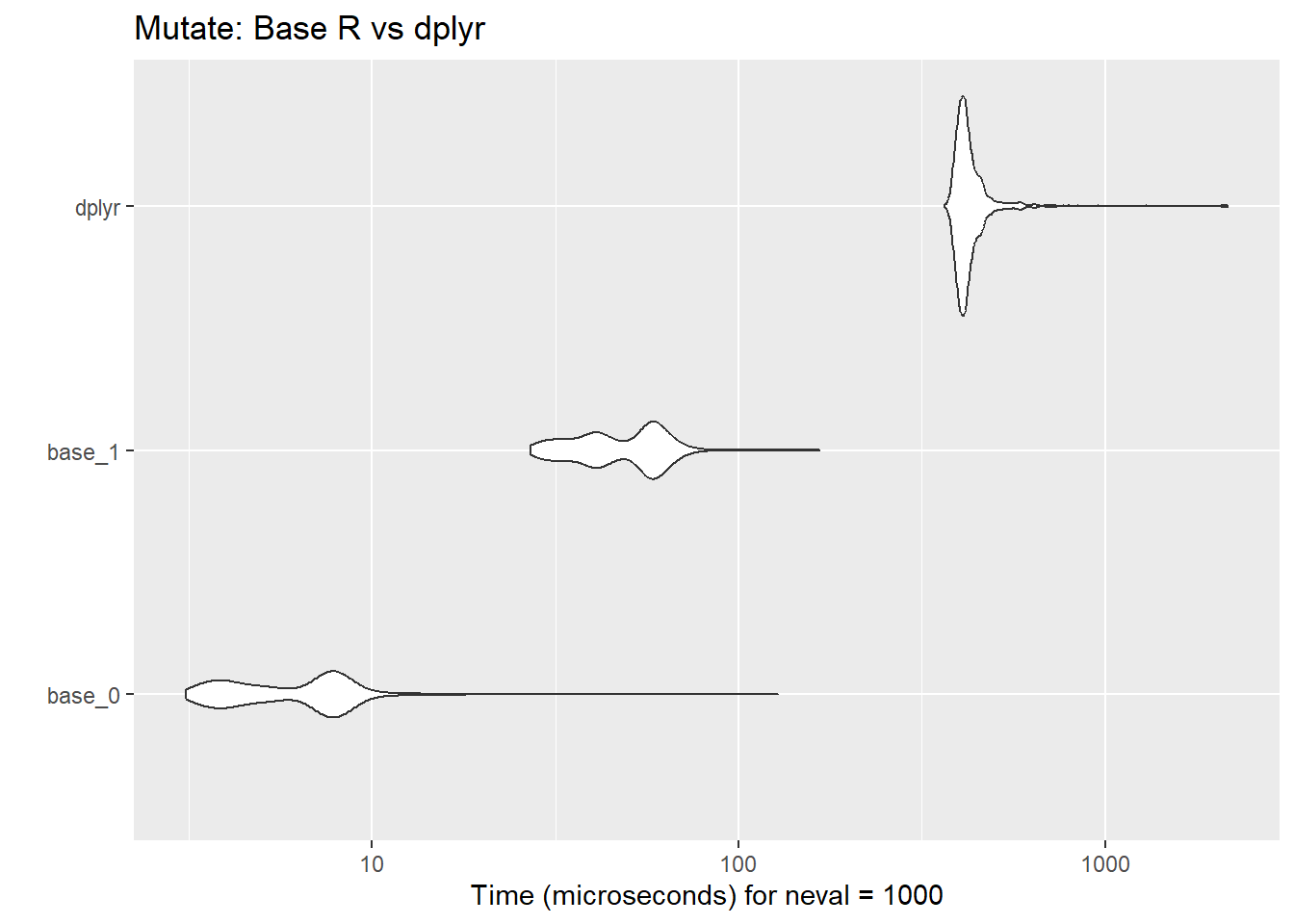
Adding or modifying columns is crucial for feature engineering. Base R provides multiple methods for this, which are benchmarked here against dplyr::mutate for their computational efficiency.
mcb_mutate <- microbenchmark(
base_0 = {iris$Sepal_LbyW <- iris$Sepal.Length / iris$Sepal.Width},
base_1 = transform(iris, Sepal_LbyW = Sepal.Length / Sepal.Width),
dplyr = mutate(iris, Sepal_LbyW = Sepal.Length / Sepal.Width),
times = 1e3
)
mcb_mutate
Unit: microseconds
   expr   min     lq     mean median     uq    max neval cld
 base_0   3.1   4.10   6.5303   6.80   8.00  127.7  1000 a
 base_1  27.0  38.65  49.2795  49.05  58.50  166.4  1000  b
  dplyr 365.4 400.85 434.6963 414.40 434.95 2154.6  1000   c
autoplot(mcb_mutate) + ggtitle("Mutate: Base R vs dplyr")
agg_mutate <- aggregate(time ~ expr, data = data.frame(mcb_mutate), mean)$time
So, base R code is on average 67 times faster than dplyr::mutate. The absolute difference in 10k simulations is 4.28166 seconds.
4. Summarise Data
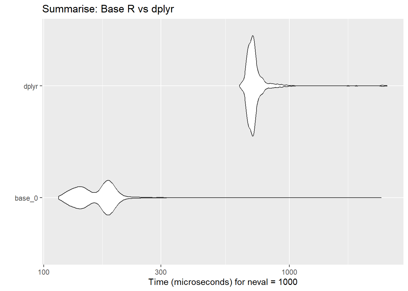
Data summarization helps derive aggregate metrics. This section compares colMeans from base R with dplyr::summarise_if, illustrating their relative performance in summarizing numeric columns.
mcb_summarise <- microbenchmark(
base_0 = with(iris, data.frame(Sepal_L_mean = mean(Sepal.Length), Sepal_W_sd = sd(Sepal.Width),
Petal_L_mean = mean(Petal.Length), Petal_W_sd = sd(Petal.Width))),
dplyr = summarise(iris, Sepal_L_mean = mean(Sepal.Length), Sepal_W_sd = sd(Sepal.Width),
Petal_L_mean = mean(Petal.Length), Petal_W_sd = sd(Petal.Width)),
times = 1e3
)
mcb_summarise
Unit: microseconds
   expr   min    lq     mean median     uq    max neval cld
 base_0 114.9 139.8 167.7646  171.7 184.95 2365.9  1000  a
  dplyr 627.7 685.1 729.6822  707.7 729.10 2497.4  1000   b
autoplot(mcb_summarise) + ggtitle("Summarise: Base R vs dplyr")
agg_summarise <- aggregate(time ~ expr, data = data.frame(mcb_summarise), mean)$time
So, base R code is on average 4 times faster than dplyr::summarise. The absolute difference in 10k simulations is 5.619176 seconds.
5. Grouped Summary
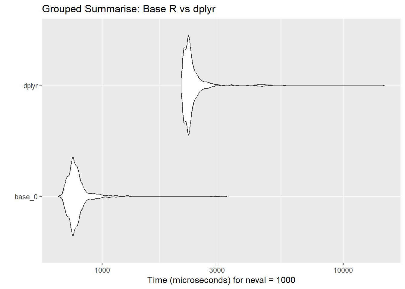
Aggregating data by groups is often required for advanced analytics. Base R’s aggregate function is tested here against dplyr’s group_by and summarise_all functions to highlight performance differences.
mcb_grp <- microbenchmark(
base_0 = aggregate(. ~ Species, data = iris, FUN = mean, na.rm = TRUE),
dplyr = iris |>
group_by(Species) |>
summarise_all(mean, na.rm = TRUE) |>
ungroup(),
times = 1e3
)
mcb_grp
Unit: microseconds
   expr    min      lq      mean median      uq     max neval cld
 base_0  657.0  741.95  795.2686  765.7  801.60  3292.2  1000  a
  dplyr 2128.8 2225.50 2392.1440 2291.4 2386.75 14798.6  1000   b
autoplot(mcb_grp) + ggtitle("Grouped Summarise: Base R vs dplyr")
agg_grp <- aggregate(time ~ expr, data = data.frame(mcb_grp), mean)$time
So, base R code is on average 3 times faster than dplyr::grp. The absolute difference in 10k simulations is 15.968754 seconds.
6. Sort Data
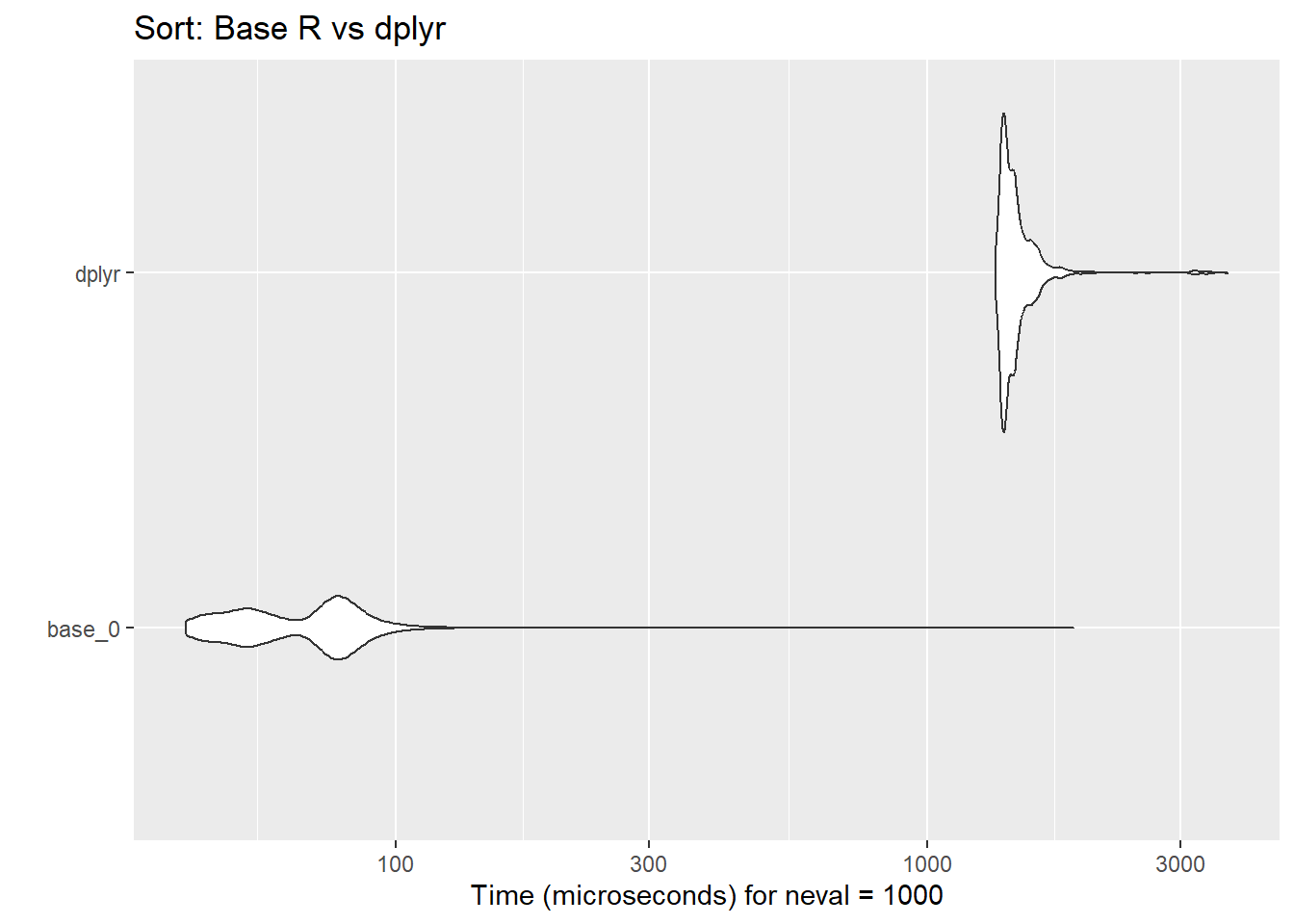
Sorting is essential for ordering data before visualization or further analysis. The benchmarks here compare the classic base R order approach to the elegant dplyr::arrange.
mcb_sort <- microbenchmark(
base_0 = iris[with(iris, order(Sepal.Length, Petal.Length)), ],
dplyr = arrange(iris, Sepal.Length, Petal.Length),
times = 1e3
)
mcb_sort
Unit: microseconds
   expr    min     lq      mean median      uq    max neval cld
 base_0   40.2   51.7   69.1362   72.8   78.95 1888.6  1000  a
  dplyr 1343.6 1392.6 1485.4011 1437.6 1498.70 3672.0  1000   b
autoplot(mcb_sort) + ggtitle("Sort: Base R vs dplyr")
agg_sort <- aggregate(time ~ expr, data = data.frame(mcb_sort), mean)$time
So, base R code is on average 21 times faster than dplyr::arrange. The absolute difference in 10k simulations is 14.162649 seconds.
7. Join Data
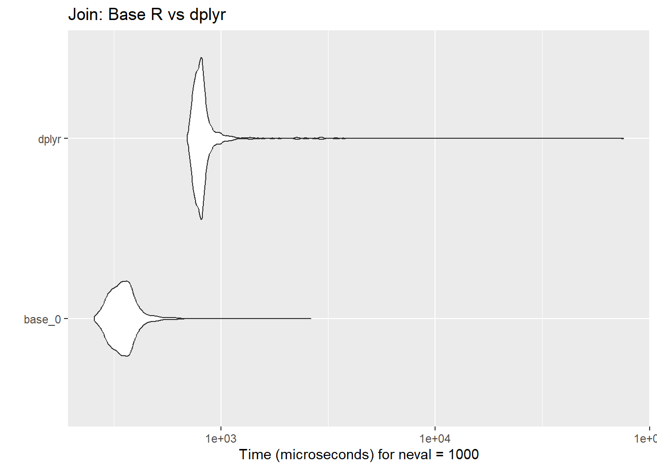
Data joins are indispensable when working with relational datasets. This section demonstrates the efficiency of base R’s merge function compared to dplyr::left_join.
iris$id <- sample.int(nrow(iris), replace = FALSE)
iris2 <- iris[sample(nrow(iris)),]
mcb_join <- microbenchmark(
base_0 = merge(iris, iris2, by = "id", all.x = TRUE),
dplyr = left_join(iris, iris2, by = "id"),
times = 1e3
)
mcb_join
Unit: microseconds
   expr   min     lq     mean median     uq     max neval cld
 base_0 256.3 313.65 357.0383 344.80 376.75  2629.4  1000  a
  dplyr 696.3 765.05 921.3512 800.45 835.75 75403.2  1000   b
autoplot(mcb_join) + ggtitle("Join: Base R vs dplyr")
agg_join <- aggregate(time ~ expr, data = data.frame(mcb_join), mean)$time
So, base R code is on average 3 times faster than dplyr::left_join. The absolute difference in 10k simulations is 5.643129 seconds.
8. Group and Apply Function 1
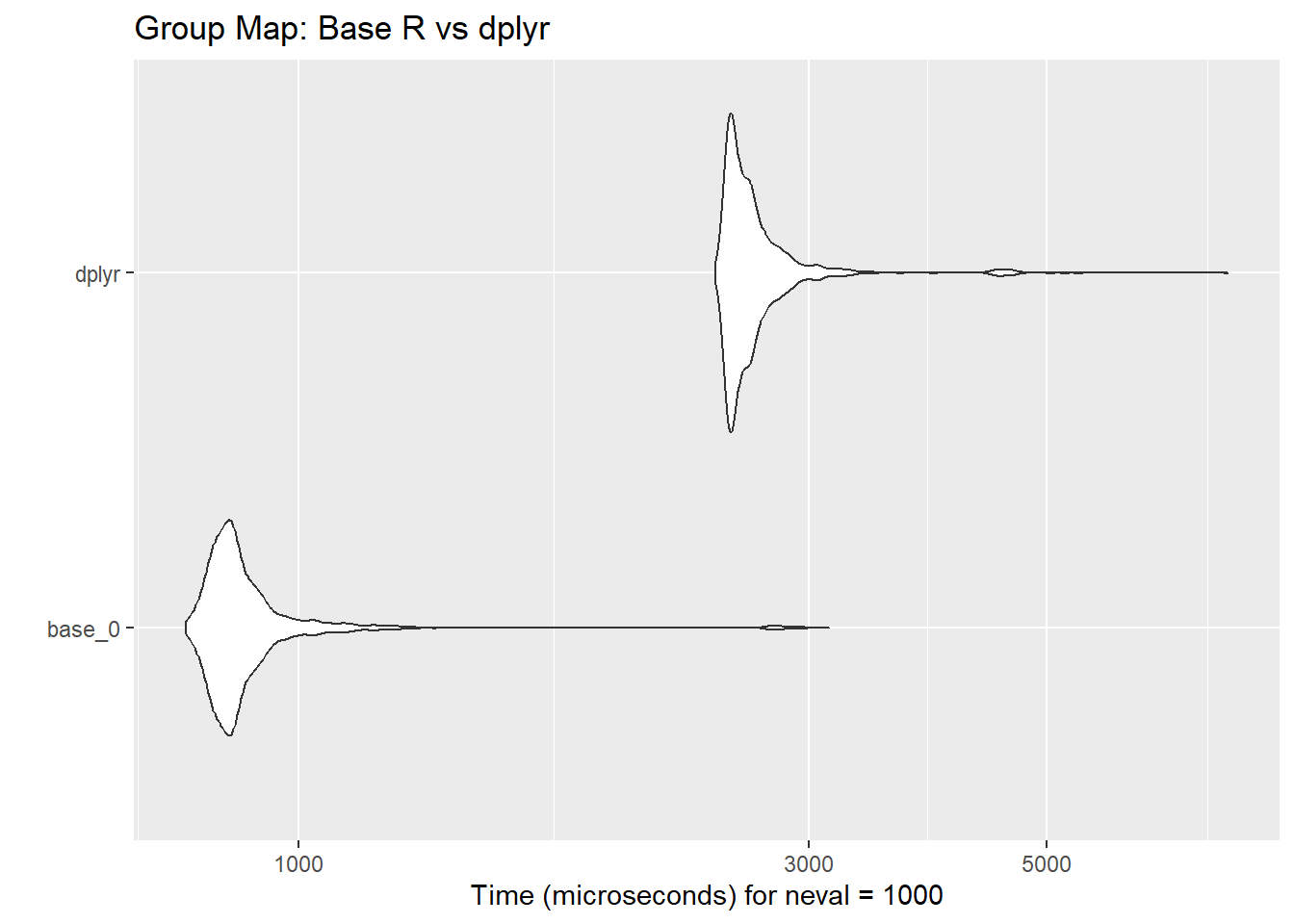
Applying models or transformations to groups of data is a frequent task in statistical workflows. This benchmark showcases the performance of split and lapply in base R versus dplyr::group_map.
mcb_grp_map <- microbenchmark(
base_0 = lapply(split(iris, iris$Species), function(x) lm(Sepal.Length ~ Petal.Length, data = x)),
dplyr = iris |>
group_by(Species) |>
group_map(~ lm(Sepal.Length ~ Petal.Length, data = .x)),
times = 1e3
)
mcb_grp_map
Unit: microseconds
   expr    min      lq      mean  median      uq    max neval cld
 base_0  784.3  840.40  911.4024  865.75  905.30 3135.7  1000  a
  dplyr 2450.7 2534.55 2684.8511 2598.80 2694.35 7384.0  1000   b
autoplot(mcb_grp_map) + ggtitle("Group Map: Base R vs dplyr")
agg_grp_map <- aggregate(time ~ expr, data = data.frame(mcb_grp_map), mean)$time
So, base R code is on average 3 times faster than dplyr::group_map. The absolute difference in 10k simulations is 17.734487 seconds.
9. Group and Apply Function 2
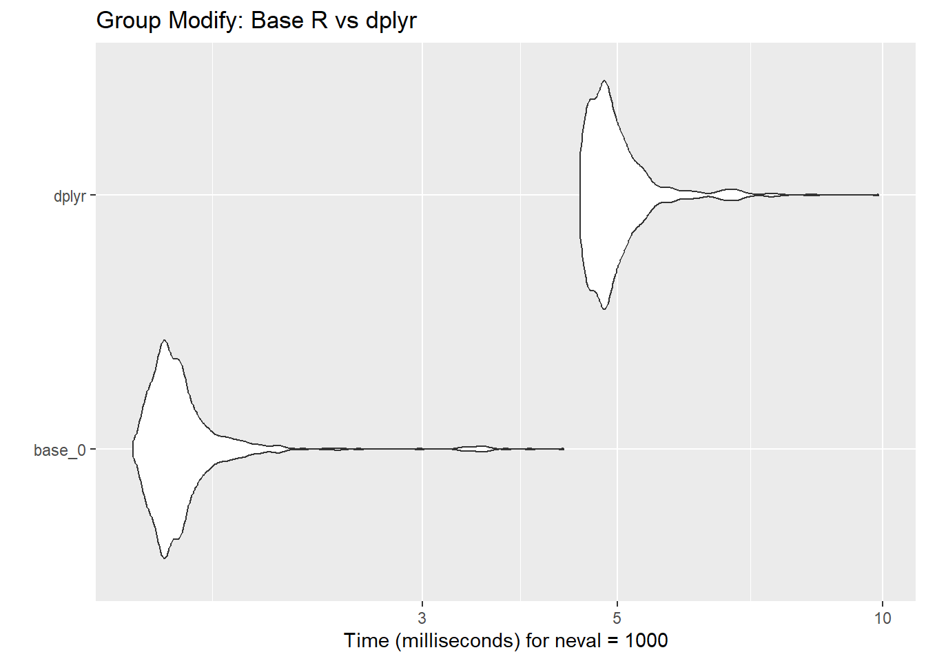
Complex operations on grouped data are common in analytical pipelines. This comparison highlights the performance of base R’s split and lapply with a row-binding step versus dplyr::group_modify.
mcb_grp_mod <- microbenchmark(
base_0 = do.call(rbind, lapply(split(iris, iris$Species), function(x)
data.frame(summary(lm(Sepal.Length ~ Petal.Length, data = x))$coefficients))),
dplyr = iris |>
group_by(Species) |>
group_modify(~ data.frame(summary(lm(Sepal.Length ~ Petal.Length, data = .x))$coefficients)) |>
ungroup(),
times = 1e3
)
mcb_grp_mod
Unit: milliseconds
   expr    min      lq     mean median      uq    max neval cld
 base_0 1.4068 1.50905 1.625191 1.5613 1.62855 4.3454  1000  a
  dplyr 4.5348 4.70640 5.007739 4.8595 5.09485 9.8918  1000   b
autoplot(mcb_grp_mod) + ggtitle("Group Modify: Base R vs dplyr")
agg_grp_mod <- aggregate(time ~ expr, data = data.frame(mcb_grp_mod), mean)$time
So, base R code is on average 3 times faster than dplyr::group_modify. The absolute difference in 10k simulations is 33.825473 seconds.
10. Rowwise
mcb_rowwise <- microbenchmark(base_0 = transform(iris,
Sepal_sd = apply(cbind(Sepal.Length, Sepal.Width), 1, sd),
Petal_sd = apply(cbind(Petal.Length, Petal.Width), 1, sd)),
dplyr = iris |>
dplyr::rowwise() |>
dplyr::mutate(Sepal_sd = sd(c(Sepal.Length, Sepal.Width)),
Petal_sd = sd(c(Petal.Length, Petal.Width))) |>
dplyr::ungroup(),
times = 1e3)
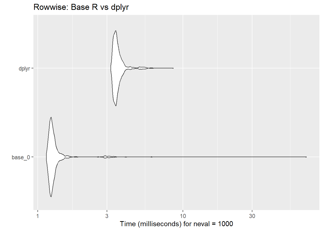
autoplot(mcb_rowwise) + ggtitle("Rowwise: Base R vs dplyr")
agg_rowwise <- aggregate(time ~ expr, data = data.frame(mcb_rowwise), mean)$time
So, base R code is on average 3 times faster than dplyr::rowwise. The absolute difference in 10k simulations is 21.835045 seconds.
11. Count Rows by Group
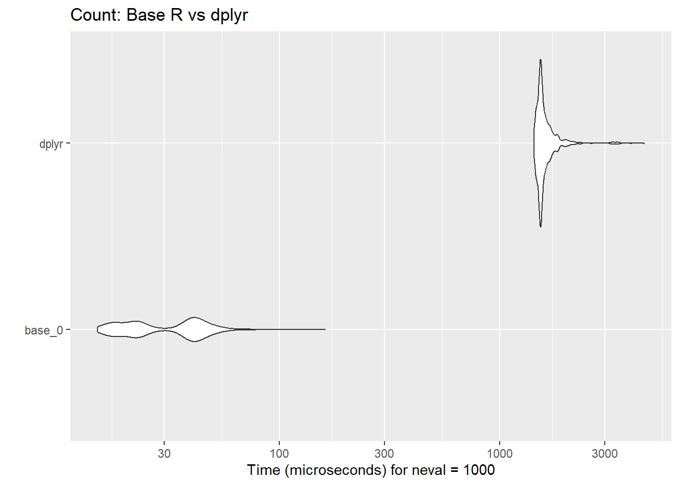
Counting the number of rows by group is a simple yet frequent operation. The comparison here emphasizes the efficiency of base R’s table function against dplyr::count.
mcb_count <- microbenchmark(
base_0 = table(iris$Species),
dplyr = iris |> count(Species),
times = 1e3
)
mcb_count
Unit: microseconds
   expr    min     lq      mean  median     uq    max neval cld
 base_0   14.9   21.3   32.3976   33.55   41.4  161.2  1000  a
  dplyr 1427.3 1516.6 1620.9624 1544.90 1639.8 4518.4  1000   b
autoplot(mcb_count) + ggtitle("Count: Base R vs dplyr")
agg_count <- aggregate(time ~ expr, data = data.frame(mcb_count), mean)$time
So, base R code is on average 50 times faster than dplyr::count. The absolute difference in 10k simulations is 15.885648 seconds.
12. Identify Distinct Rows
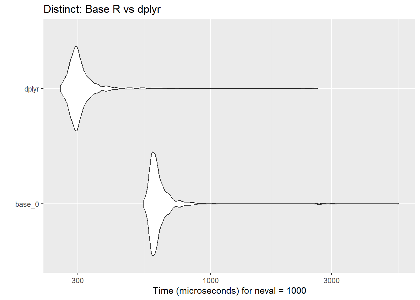
Identifying unique rows is crucial for deduplication. This benchmark compares base R’s unique function with dplyr::distinct, shedding light on performance differences for this operation.
mcb_distinct <- microbenchmark(
base_0 = unique(rbind(iris, iris)),
dplyr = distinct(rbind(iris, iris)),
times = 1e3
)
mcb_distinct
Unit: microseconds
   expr   min     lq     mean median     uq    max neval cld
 base_0 546.6 587.15 644.9276  607.2 640.95 5494.7  1000  a
  dplyr 255.9 285.75 315.5954  297.9 315.00 2635.5  1000   b
autoplot(mcb_distinct) + ggtitle("Distinct: Base R vs dplyr")
agg_distinct <- aggregate(time ~ expr, data = data.frame(mcb_distinct), mean)$time
So, base R code is on average 2 times slower than dplyr::distinct. The absolute difference in 10k simulations is 3.293322 seconds.
Summary
Given that these functions are very commonly used, it is fair to assume that these functions are used at least 5 times in a standard simulation code. If that simulation is repeated for 10k times, then the total gain we have by using base R is at least 11.7210869 minutes.
Conclusion
This analysis demonstrates
- that while dplyr offers user-friendly functions and a consistent syntax,
- base R can often be faster for basic operations, especially with large datasets.
The choice between base R and dplyr should consider both readability and computational efficiency, dependent on the scale and complexity of your data tasks.
- For intensive data simulations, careful function choice can lead to significant performance gains,
- underscoring the importance of benchmarking and profiling in the R language.