Introduction

Ensemble learning is a powerful way to combine multiple machine learning models to boost predictive performance. The SuperLearner R package is a go-to for this, however it only supports gaussian or binomial to describe the error distribution. Using the clean, flexible tidymodels framework we can implement these functionalities and also extend it for multi-class classification, count data regression. In this post, I’ll walk you through how to build a SuperLearner-style ensemble model with tidymodels, keeping things lucid and practical. We’ll cover the key steps, share reusable code, and apply it to real datasets for binary classification, count regression, standard regression, and multi-class classification.

Why Tidymodels for Ensemble Learning?

The SuperLearner package is great, but tidymodels offers a modular, intuitive workflow that’s perfect for building and tuning ensembles. With packages like recipes, workflows, and stacks, you can preprocess data, define models, and stack them into a robust ensemble with ease. Plus, tidymodels integrates seamlessly with modern R tools, making your code clean and reproducible.

Let’s dive into the process with a clear roadmap and examples you can adapt for your own projects.

Packages You’ll Need

First, let’s load the essential packages. These cover everything from data preprocessing to model stacking and evaluation.

library(tidymodels, quietly = TRUE)

## Warning: package 'tidymodels' was built under R version 4.5.1

## ── Attaching packages ────────────────────────────────────── tidymodels 1.3.0 ──

## ✔ broom        1.0.9     ✔ recipes      1.3.1
## ✔ dials        1.4.1     ✔ rsample      1.3.0
## ✔ dplyr        1.1.4     ✔ tibble       3.2.1
## ✔ ggplot2      3.5.2     ✔ tidyr        1.3.1
## ✔ infer        1.0.9     ✔ tune         1.3.0
## ✔ modeldata    1.5.0     ✔ workflows    1.2.0
## ✔ parsnip      1.3.2     ✔ workflowsets 1.1.1
## ✔ purrr        1.0.4     ✔ yardstick    1.3.2

## Warning: package 'broom' was built under R version 4.5.1

## Warning: package 'dials' was built under R version 4.5.1

## Warning: package 'infer' was built under R version 4.5.1

## Warning: package 'modeldata' was built under R version 4.5.1

## Warning: package 'parsnip' was built under R version 4.5.1

## Warning: package 'recipes' was built under R version 4.5.1

## Warning: package 'tune' was built under R version 4.5.1

## Warning: package 'workflows' was built under R version 4.5.1

## Warning: package 'workflowsets' was built under R version 4.5.1

## Warning: package 'yardstick' was built under R version 4.5.1

## ── Conflicts ───────────────────────────────────────── tidymodels_conflicts() ──
## ✖ purrr::discard() masks scales::discard()
## ✖ dplyr::filter()  masks stats::filter()
## ✖ dplyr::lag()     masks stats::lag()
## ✖ recipes::step()  masks stats::step()

library(stacks)

## Warning: package 'stacks' was built under R version 4.5.1

library(discrim)      # For quadratic discriminant analysis (QDA)

## Warning: package 'discrim' was built under R version 4.5.1

## 
## Attaching package: 'discrim'

## The following object is masked from 'package:dials':
## 
##     smoothness

library(poissonreg)   # For Poisson regression

## Warning: package 'poissonreg' was built under R version 4.5.1

set.seed(123)         # For reproducibility

The Four-Step Process

Building a SuperLearner with tidymodels boils down to four high-level steps. Think of it as a recipe for ensemble success:

Step 1: Prep Your Data with a Recipe

Use the recipes package to preprocess your data. This ensures all predictors are ready for modeling (e.g., converting categorical variables to dummy variables and removing zero-variance predictors). Of course, you can add more based on your needs and what makes sense.

data_rec <- recipe(as.formula(formula), data = data) |>
  step_dummy(all_nominal_predictors()) |>
  step_zv(all_predictors())

Step 2: Build a Workflow

Create a workflow that combines your data recipe with a model specification. For example, if you’re using XGBoost, it might look like this:

wflow <- workflow() |>
  add_recipe(data_rec) |>
  add_model(boost_spec)  # Example: XGBoost model spec

Step 3: Tune Your Models

Tune each model’s hyperparameters using cross-validation. This step optimizes each algorithm’s performance before stacking.

tune_results <- tune_grid(
  object = wflow,
  resamples = folds,
  grid = 10,
  control = control_stack_grid()
)

Step 4: Stack the Models

Combine your tuned models into an ensemble using the stacks package. This blends their predictions and fits the final ensemble.

ensemble_model <- stacks() |>
  add_candidates(do.call(as_workflow_set, member_list)) |>
  blend_predictions() |>
  fit_members()

A Reusable Function for Tidymodels SuperLearner

To make this process reusable, I’ve crafted a function that automates the workflow for various model types (e.g., XGBoost, random forest, neural networks) and problem types (binary classification, regression, count data, or multi-class classification). Here’s the polished version:

sl_tidy_workflow <- function(member, mode) {
  if (member == "poisson") {
    mod_spec <- poisson_reg() |>
      set_mode(mode) |>
      set_engine("glm")
  } else if (member == "elasto_poisson") {
    mod_spec <- poisson_reg(penalty = tune(), mixture = tune()) |>
      set_mode(mode) |>
      set_engine("glmnet")
  } else if (member == "poisson_zero") {
    mod_spec <- poisson_reg() |>
      set_mode(mode) |>
      set_engine("zeroinfl")
  } else if (member == "multi") {
    mod_spec <- multinom_reg(penalty = tune()) |>
      set_mode(mode) |>
      set_engine("nnet")
  } else if (member == "elasto_multi") {
    mod_spec <- multinom_reg(penalty = tune(), mixture = tune()) |>
      set_mode(mode) |>
      set_engine("glmnet")
  } else if (member == "knn") {
    mod_spec <- nearest_neighbor(neighbors = tune(), weight_func = tune(), dist_power = tune()) |>
      set_mode(mode) |>
      set_engine("kknn")
  } else if (member == "boost") {
    mod_spec <- boost_tree(mtry = tune(), min_n = tune(), trees = 500) |>
      set_mode(mode) |>
      set_engine("xgboost")
  } else if (member == "rf") {
    mod_spec <- rand_forest(mtry = tune(), min_n = tune(), trees = 500) |>
      set_mode(mode) |>
      set_engine("ranger")
  } else if (member == "nnet") {
    mod_spec <- mlp(hidden_units = tune(), penalty = tune(), epochs = tune()) |>
      set_mode(mode) |>
      set_engine("nnet")
  } else if (member == "logit") {
    mod_spec <- logistic_reg() |>
      set_mode(mode) |>
      set_engine("glm")
  } else if (member == "lm") {
    mod_spec <- linear_reg() |>
      set_mode(mode) |>
      set_engine("lm")
  } else if (member == "elasto_logit") {
    mod_spec <- logistic_reg(penalty = tune(), mixture = tune()) |>
      set_mode(mode) |>
      set_engine("glmnet")
  } else if (member == "elasto_lm") {
    mod_spec <- linear_reg(penalty = tune(), mixture = tune()) |>
      set_mode(mode) |>
      set_engine("glmnet")
  } else if (member == "qda") {
    mod_spec <- discrim_quad() |>
      set_mode(mode) |>
      set_engine("MASS")
  } else if (member == "lsvm") {
    mod_spec <- svm_linear() |>
      set_mode(mode) |>
      set_engine("kernlab")
  } else if (member == "psvm") {
    mod_spec <- svm_poly() |>
      set_mode(mode) |>
      set_engine("kernlab")
  } else if (member == "rsvm") {
    mod_spec <- svm_rbf() |>
      set_mode(mode) |>
      set_engine("kernlab")
  }
  return(mod_spec)
}

Now, let us implement the above mentioned 4 steps.

sl_tidy <- function(formula, data, sl_lib = NULL, cv_v = 5, mode = "bin") {
  # Check for required packages
  req_pkg_list <- c("xgboost", "ranger", "nnet", "earth", "stats", "glmnet", "discrim", "kernlab", "kknn", "mgcv", "poissonreg", "mlbench", "COUNT", "pscl")
  not_installed_pkgs <- setdiff(req_pkg_list, installed.packages()[, 1])
  if (length(not_installed_pkgs)) {
    stop(paste0("Please install: install.packages(c('", paste(not_installed_pkgs, collapse = "','"), "'))"))
  }

  # Define model libraries for different modes
  sl_lib_cl <- c("boost", "rf", "nnet", "logit", "elasto_logit", "qda", "lsvm", "psvm", "rsvm")
  sl_lib_reg <- c("boost", "lm", "elasto_lm", "nnet", "knn", "rf", "lsvm", "psvm", "rsvm")
  sl_lib_multi <- c("boost", "rf", "multi", "elasto_multi", "qda", "lsvm", "psvm", "rsvm")
  sl_lib_count <- c("boost", "knn", "rf", "lsvm", "psvm", "rsvm", "poisson", "elasto_poisson")

  # Set mode and model library
  if (mode == "bin") {
    mode <- "classification"
    sl_lib_master <- sl_lib_cl
  } else if (mode == "cont") {
    mode <- "regression"
    sl_lib_master <- sl_lib_reg
  } else if (mode == "multi") {
    mode <- "classification"
    sl_lib_master <- sl_lib_multi
  } else if (mode == "count") {
    mode <- "regression"
    sl_lib_master <- sl_lib_count
  }

  if (is.null(sl_lib)) {
    sl_lib <- sl_lib_master
  } else if (!all(sl_lib %in% sl_lib_master)) {
    stop(paste0("'sl_lib' must be one of: ", paste(sl_lib_master, collapse = ", ")))
  }

  # Step 1: Create recipe
  data_rec <- recipe(as.formula(formula), data = data) |>
    step_dummy(all_nominal_predictors()) |>
    step_zv(all_predictors())

  # Step 2: Initialize workflow
  data_wflow <- workflow() |>
    add_recipe(data_rec)

  # Step 3: Cross-validation folds
  if (mode == "classification") {
    folds <- vfold_cv(data, v = cv_v, strata = as.character(formula)[2])
  } else {
    folds <- vfold_cv(data, v = cv_v)
  }

  # Tune models
  member_list <- lapply(sl_lib, function(member) {
    mod_spec <- sl_tidy_workflow(member = member, mode = mode)
    mod_wflow <- data_wflow |> add_model(mod_spec)
    mod_res <- tryCatch(
      suppressWarnings(tune_grid(
        object = mod_wflow,
        resamples = folds,
        grid = 10,
        control = control_stack_grid()
      )),
      error = function(e) NULL
    )
    if (!is.null(mod_res)) {
      cat(paste0("Tuned ", member, " model\n"))
    }
    return(mod_res)
  })
  names(member_list) <- sl_lib
  member_list <- member_list[lengths(member_list) != 0]

  # Step 4: Stack models
  data_model_st <- stacks()
  for (res in names(member_list)) {
    data_model_st <- data_model_st |>
      add_candidates(member_list[[res]], name = res)
  }

  data_model_st <- data_model_st |>
    blend_predictions() |>
    fit_members()

  return(data_model_st)
}

Real-World Examples

Let’s see this in action with four datasets, covering binary classification, count regression, standard regression, and multi-class classification. Each dataset is chosen to demonstrate the flexibility of our tidymodels SuperLearner approach, and I’ll provide some context about each to help you understand their relevance.

Binary Classification: Pima Indians Diabetes

The PimaIndiansDiabetes2 dataset, from the mlbench package, contains medical data on Pima Indian women, including variables like glucose levels, blood pressure, and body mass index (BMI). The goal is to predict diabetes status (positive or negative), making it a classic binary classification problem. This dataset is widely used in machine learning to study diagnostic prediction models, as it reflects real-world medical data with some missing values and class imbalance.

data("PimaIndiansDiabetes2", package = "mlbench")
diabetes_data <- PimaIndiansDiabetes2 |>
  na.omit() |>
  mutate(diabetes = factor(if_else(diabetes == "pos", 1, 0)))
head(diabetes_data)

##    pregnant glucose pressure triceps insulin mass pedigree age diabetes
## 4         1      89       66      23      94 28.1    0.167  21        0
## 5         0     137       40      35     168 43.1    2.288  33        1
## 7         3      78       50      32      88 31.0    0.248  26        1
## 9         2     197       70      45     543 30.5    0.158  53        1
## 14        1     189       60      23     846 30.1    0.398  59        1
## 15        5     166       72      19     175 25.8    0.587  51        1

Let’s split the data into training and test sets.

diabetes_split <- initial_split(diabetes_data, prop = 0.8, strata = "diabetes")
diabetes_train <- training(diabetes_split)
diabetes_test <- testing(diabetes_split)

Let’s now build the superlearner

diabetes_SL <- sl_tidy(diabetes ~ ., data = diabetes_train, cv_v = 5, mode = "bin")

## i Creating pre-processing data to finalize unknown parameter: mtry

## Tuned boost model

## i Creating pre-processing data to finalize unknown parameter: mtry

## Tuned rf model
## Tuned nnet model
## Tuned logit model
## Tuned elasto_logit model
## Tuned qda model
## Tuned lsvm model
## Tuned psvm model
## Tuned rsvm model

## Warning: Predictions from 2 candidates were identical to those from existing candidates
## and were removed from the data stack.

##  Setting default kernel parameters

## Warning: package 'future' was built under R version 4.5.1

Use the superlearner for prediction

# Predict
diabetes_test_pred <- diabetes_test %>%
  bind_cols(predict(diabetes_SL, ., type = "prob"))

Evaluate the ROC AUC

# Evaluate with ROC AUC
library(pROC)

## Type 'citation("pROC")' for a citation.

## 
## Attaching package: 'pROC'

## The following objects are masked from 'package:stats':
## 
##     cov, smooth, var

diabetes_roc <- roc(response = diabetes_test_pred$diabetes, predictor = diabetes_test_pred$.pred_1)

## Setting levels: control = 0, case = 1

## Setting direction: controls < cases

auc(diabetes_roc)

## Area under the curve: 0.8106

ggroc(diabetes_roc) +
  theme_minimal()

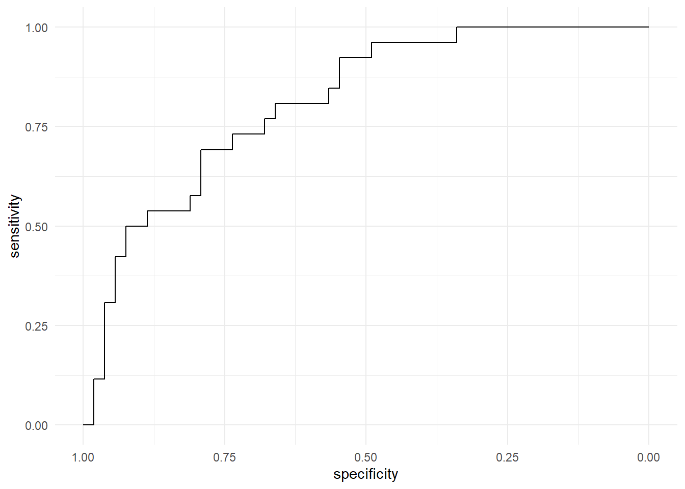
This gives you a model that predicts diabetes with a stacked ensemble, and the ROC curve visualizes its performance in distinguishing between diabetic and non-diabetic cases.

Count Data Regression: Epileptic Seizures

The epil dataset, from the MASS package, records the number of epileptic seizures in patients over time, along with predictors like treatment type and baseline seizure counts. It’s a great example for count regression, as seizure counts are non-negative integers with potential overdispersion, making Poisson. This dataset is often used to study count data in medical research.

data("epil", package = "MASS")
epil_data <- epil |> na.omit() |> dplyr::select(-subject)
head(epil_data)

##   y     trt base age V4 period      lbase       lage
## 1 5 placebo   11  31  0      1 -0.7563538 0.11420370
## 2 3 placebo   11  31  0      2 -0.7563538 0.11420370
## 3 3 placebo   11  31  0      3 -0.7563538 0.11420370
## 4 3 placebo   11  31  1      4 -0.7563538 0.11420370
## 5 3 placebo   11  30  0      1 -0.7563538 0.08141387
## 6 5 placebo   11  30  0      2 -0.7563538 0.08141387

Let’s split the data into training and test sets.

epil_split <- initial_split(epil_data, prop = 0.8)
epil_train <- training(epil_split)
epil_test <- testing(epil_split)

Let’s now build the superlearner

epil_SL <- sl_tidy(y ~ ., data = epil_train, cv_v = 5, mode = "count")

## i Creating pre-processing data to finalize unknown parameter: mtry

## Tuned boost model
## Tuned knn model

## i Creating pre-processing data to finalize unknown parameter: mtry

## Tuned rf model
## Tuned lsvm model
## Tuned psvm model
## Tuned rsvm model
## Tuned poisson model
## Tuned elasto_poisson model
##  Setting default kernel parameters  
##  Setting default kernel parameters

Use the superlearner for prediction

# Predict
epil_test_pred <- epil_test %>%
  bind_cols(predict(epil_SL, ., type = "numeric"))

Now visualize

# Visualize
ggplot(epil_test_pred, aes(x = y, y = round(.pred))) +
  geom_point() +
  labs(x = "Observed Seizure Counts", y = "Predicted Seizure Counts") +
  theme_minimal()

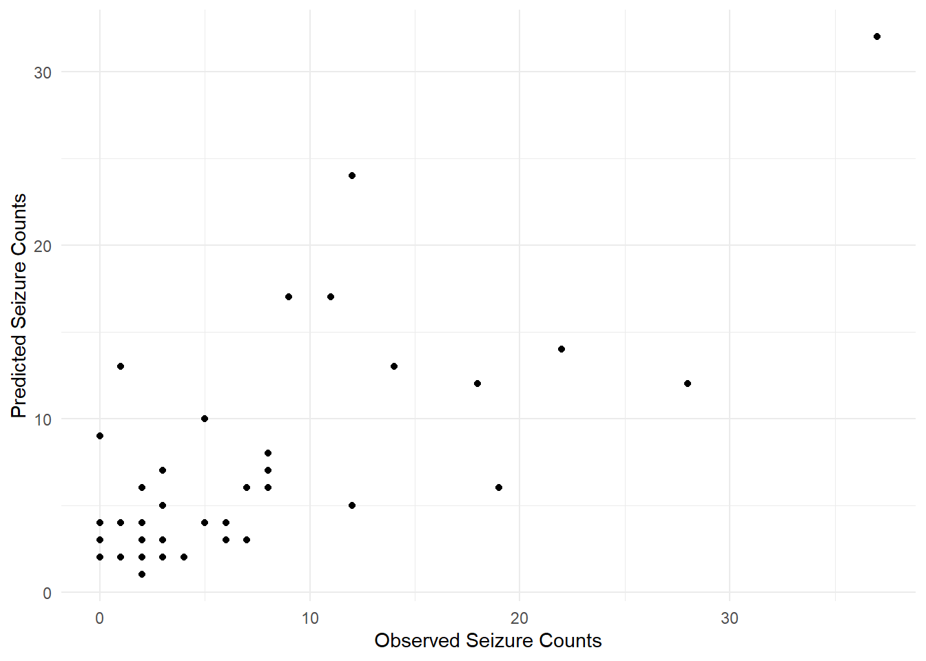
The scatter plot shows how well our ensemble predicts seizure counts, useful for evaluating treatment effects in epilepsy studies.

Regression: Birthweight Prediction

The birthwt dataset, also from the MASS package, contains data on infant birthweights and maternal factors like smoking status, age, and weight. It’s a standard dataset for regression tasks, as birthweight is a continuous outcome influenced by multiple predictors. This dataset is valuable for studying maternal and fetal health, often used in statistical modeling to explore risk factors for low birthweight.

data("birthwt", package = "MASS")
bwt_data <- birthwt |> na.omit()
head(bwt_data)

##    low age lwt race smoke ptl ht ui ftv  bwt
## 85   0  19 182    2     0   0  0  1   0 2523
## 86   0  33 155    3     0   0  0  0   3 2551
## 87   0  20 105    1     1   0  0  0   1 2557
## 88   0  21 108    1     1   0  0  1   2 2594
## 89   0  18 107    1     1   0  0  1   0 2600
## 91   0  21 124    3     0   0  0  0   0 2622

Let’s split the data into training and test sets.

bwt_split <- initial_split(bwt_data, prop = 0.8)
bwt_train <- training(bwt_split)
bwt_test <- testing(bwt_split)

And then Build the superlearner

bwt_SL <- sl_tidy(bwt ~ ., data = bwt_train, cv_v = 5, mode = "cont")

## i Creating pre-processing data to finalize unknown parameter: mtry

## Tuned boost model
## Tuned lm model
## Tuned elasto_lm model

## → A | warning: A correlation computation is required, but `estimate` is constant and has 0
##                standard deviation, resulting in a divide by 0 error. `NA` will be returned.

## 
There were issues with some computations   A: x1

There were issues with some computations   A: x2

There were issues with some computations   A: x3

There were issues with some computations   A: x4

There were issues with some computations   A: x5

There were issues with some computations   A: x5

## Tuned nnet model
## Tuned knn model

## i Creating pre-processing data to finalize unknown parameter: mtry

## Tuned rf model
## Tuned lsvm model
## Tuned psvm model
## Tuned rsvm model

## Warning: The inputted `candidates` argument `nnet` generated notes during
## tuning/resampling. Model stacking may fail due to these issues; see
## `collect_notes()` (`?tune::collect_notes()`) if so.

Now, use it for prediction

# Predict
bwt_test_pred <- bwt_test %>%
  bind_cols(predict(bwt_SL, ., type = "numeric"))

We can then visualize as follows:

# Visualize
ggplot(bwt_test_pred, aes(x = bwt, y = round(.pred))) +
  geom_point() +
  labs(x = "Observed Birthweight (grams)", y = "Predicted Birthweight (grams)") +
  theme_minimal()

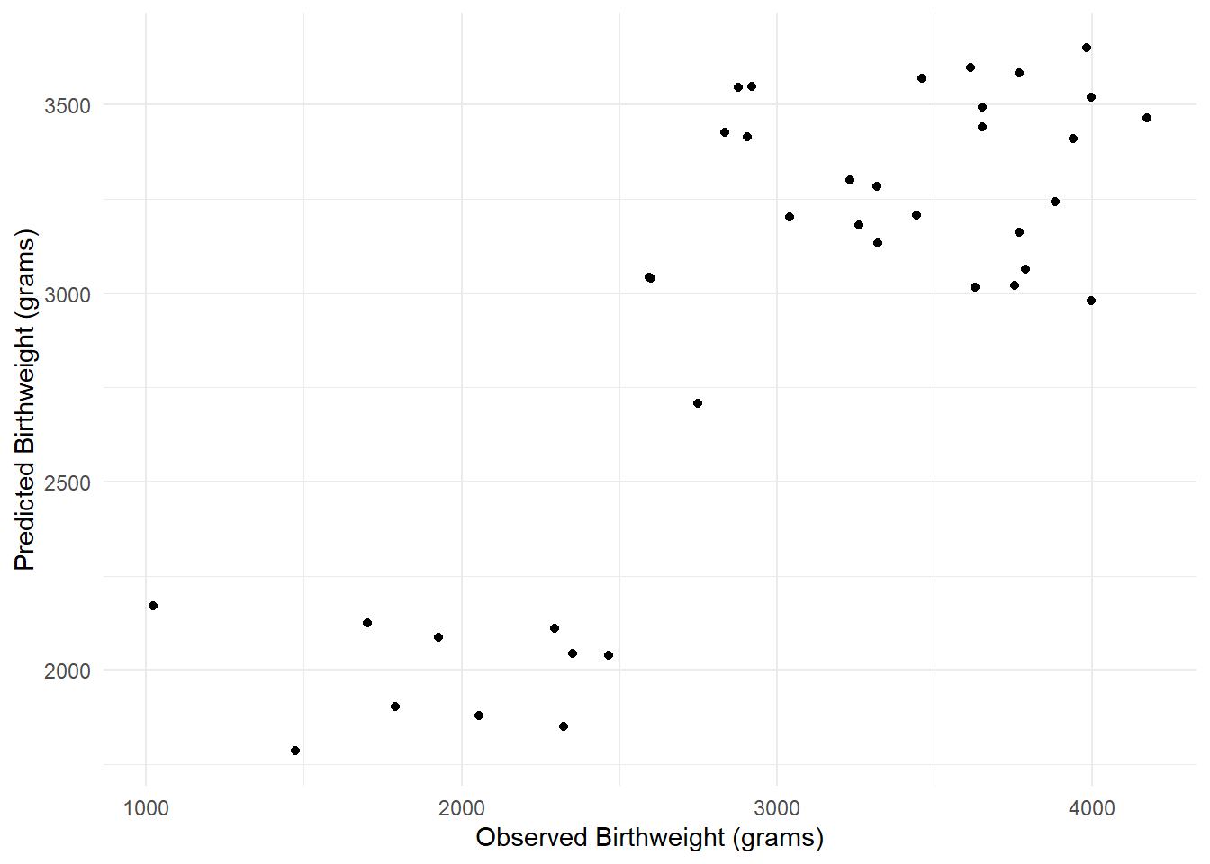
This shows how the ensemble performs in predicting birthweight, which can inform medical interventions for at-risk pregnancies.

Multi-Class Classification: Iris Species

The iris dataset, from the datasets package, is a classic in machine learning. It includes measurements of sepal and petal dimensions for three iris species: setosa, versicolor, and virginica. With four continuous predictors and three classes, it’s perfect for multi-class classification. This dataset, introduced by Ronald Fisher, remains a benchmark for testing classification algorithms due to its simplicity and clear class separation.

data("iris", package = "datasets")
species_data <- iris |> na.omit()
head(species_data)

##   Sepal.Length Sepal.Width Petal.Length Petal.Width Species
## 1          5.1         3.5          1.4         0.2  setosa
## 2          4.9         3.0          1.4         0.2  setosa
## 3          4.7         3.2          1.3         0.2  setosa
## 4          4.6         3.1          1.5         0.2  setosa
## 5          5.0         3.6          1.4         0.2  setosa
## 6          5.4         3.9          1.7         0.4  setosa

We split it into training and test sets:

species_split <- initial_split(species_data, prop = 0.8, strata = "Species")
species_train <- training(species_split)
species_test <- testing(species_split)

Build the superlearner

species_SL <- sl_tidy(Species ~ ., data = species_train, cv_v = 5, mode = "multi")

## i Creating pre-processing data to finalize unknown parameter: mtry

## Tuned boost model

## i Creating pre-processing data to finalize unknown parameter: mtry

## Tuned rf model
## Tuned multi model
## Tuned elasto_multi model
## Tuned qda model
## Tuned lsvm model
## Tuned psvm model
## Tuned rsvm model

## Warning: Predictions from 14 candidates were identical to those from existing candidates
## and were removed from the data stack.

## Warning: Predictions from 3 candidates were identical to those from existing candidates
## and were removed from the data stack.

##  Setting default kernel parameters

Use it for prediction

# Predict
species_test_pred <- species_test %>%
  bind_cols(predict(species_SL, ., type = "prob"))

Evaluate the ROC

# Evaluate with multi-class ROC
species_roc <- multiclass.roc(
  response = species_test_pred$Species,
  predictor = cbind(
    setosa = species_test_pred$.pred_setosa,
    versicolor = species_test_pred$.pred_versicolor,
    virginica = species_test_pred$.pred_virginica
  )
)
auc(species_roc)

## Multi-class area under the curve: 1

This evaluates the ensemble’s ability to distinguish between iris species, a task relevant to botanical classification and algorithm benchmarking.

Wrapping Up

Using tidymodels, you can build a SuperLearner-style ensemble that’s flexible, reproducible, and easy to understand. The sl_tidy function simplifies the process, letting you focus on modeling rather than boilerplate code. Whether you’re tackling medical diagnostics (Pima Indians Diabetes), count data (epileptic seizures), health outcomes (birthweight), or classic classification (iris), this approach scales to your needs. Based on github conversations, support for censored regression is coming in stacks, which will enable extension of this for time-to-event data.

Try it out on your own dataset, tweak the model library, and see how stacking can boost your predictions.

💬 Like this blog? Share your thoughts and use-cases on LinkedIn and tag me!